Working with Kernels
This notebook is meant as a basic walk through of how to use kernels with squidward models. Squidward was built to be a flexible Gaussian process modeling package. Many GP modeling packages sarcifice a great deal of flexibility for gains in performance and/or simplicity. Squidward is meant to be a “make your own adventure” model building package.
Using Default Kernels
Optimized Kernels
There are a variety of default kernels that you can choose to use. Those coded for optimal performance can be found in the optimized_kernels module. These kernels tend to be very vanilla and inflexible, but run much more efficiently than other options. below is an example of how to use an optimized kernel:
[3]:
import numpy as np
import matplotlib.pyplot as plt

from squidward.kernels import optimized_kernels
[4]:
# Call help if you are uncertain about the kernel parameters

help(optimized_kernels.RBF_Kernel)
Help on class RBF_Kernel in module squidward.kernels.optimized_kernels:

class RBF_Kernel(builtins.object)
 |  Radial Basis Function Kernel
 |
 |  Methods defined here:
 |
 |  __call__(self, alpha, beta)
 |      Description
 |      ----------
 |      Calls the kernel object.
 |
 |      Parameters
 |      ----------
 |      alpha: array_like
 |          The first vector to compare.
 |      beta: array_like
 |          The second vector to compare.
 |
 |      Returns
 |      ----------
 |      A array representing the covariance between points in
 |      the vectors alpha and beta.
 |
 |  __init__(self, lengthscale, var_k)
 |      Description
 |      ----------
 |      Radial basis function (rbf) kernel.
 |
 |      Parameters
 |      ----------
 |      lengthscale: Float
 |          The lengthscale of the rbf function that detrmins the radius around
 |          which the value of an observation imapcts other observations.
 |      var_k: Float
 |          The kernel variance or amplitude. This can be thought of as the maximum
 |          value that the rbf function can take.
 |
 |      Returns
 |      ----------
 |      kernel object
 |
 |  ----------------------------------------------------------------------
 |  Data descriptors defined here:
 |
 |  __dict__
 |      dictionary for instance variables (if defined)
 |
 |  __weakref__
 |      list of weak references to the object (if defined)
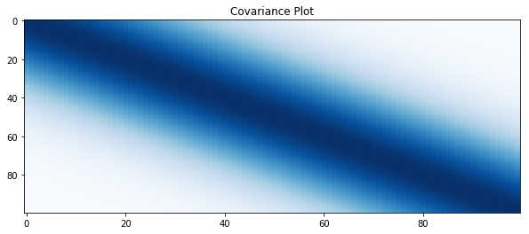
[5]:
# create kernel object
kernel = optimized_kernels.RBF_Kernel(lengthscale=1.0, var_k=2.0**2)
[19]:
# create a vector
alpha = np.linspace(-2.0, 2.0, 100)
# get covariance
covariance = kernel(alpha, alpha)
[7]:
# plot covariance
plt.figure(figsize=(10, 4))
plt.title("Covariance Plot")
plt.imshow(covariance, cmap='Blues', interpolation='nearest', aspect='auto')
plt.show()
Flexible Kernels
If the optimized kernels don’t meet your needs, squidward allows for the creation of customer kernels. We demonstrate three examples of how this can be done below in order of complexity. The idea behind this framework is to make it possible to use any possible valid kernel that you might want to use.
These kernels will be comprised of two parts. The first is a distance function that defines the distance between two vectors (each vector represents a single observation):
The second part applies this distance function to every combination of points in the two observation sets that are being compared:
The examples are broken down into: 1. Basic Use 2. Combining Kernels 3. Making A New Kernel
1) Basic Use
[8]:
from squidward.kernels import distance, kernel_base
[9]:
# Call help if you are uncertain about the distance function parameters

help(distance.RBF)
Help on class RBF in module squidward.kernels.distance:

class RBF(builtins.object)
 |  Class for radial basis fucntion distance measure.
 |
 |  Methods defined here:
 |
 |  __call__(self, alpha, beta)
 |      Description
 |      ----------
 |      Calls the kernel object.
 |
 |      Parameters
 |      ----------
 |      alpha: array_like
 |          The first vector to compare.
 |      beta: array_like
 |          The second vector to compare.
 |
 |      Returns
 |      ----------
 |      A array representing the covariance between points in
 |      the vectors alpha and beta.
 |
 |  __init__(self, lengthscale, var_k)
 |      Description
 |      ----------
 |      Radial basis function (rbf) distance measure between vectors/arrays.
 |
 |      Parameters
 |      ----------
 |      lengthscale: Float
 |          The lengthscale of the rbf function that detrmins the radius around
 |          which the value of an observation imapcts other observations.
 |      var_k: Float
 |          The kernel variance or amplitude. This can be thought of as the maximum
 |          value that the rbf function can take.
 |
 |      Returns
 |      ----------
 |      distance object
 |
 |  ----------------------------------------------------------------------
 |  Data descriptors defined here:
 |
 |  __dict__
 |      dictionary for instance variables (if defined)
 |
 |  __weakref__
 |      list of weak references to the object (if defined)
[14]:
# define the distance function
distance_function = distance.RBF(lengthscale=1.0, var_k=2.0**2)
# define the kernel
# the kernel comes with two 'methods' k1 and k2
# k2 is optimized to run faster for use cases
# where the GP is fit repeatedly
kernel = kernel_base.Kernel(distance_function=distance_function, method="k1")
[15]:
# create a vector
alpha = np.linspace(-2.0, 2.0, 100)
# get covariance
covariance = kernel(alpha, alpha)
[16]:
# plot covariance
plt.figure(figsize=(10, 4))
plt.title("Covariance Plot")
plt.imshow(covariance, cmap='Blues', interpolation='nearest', aspect='auto')
plt.show()

2) Combining Kernels
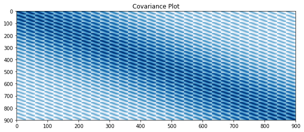
Imagine that the observations that we want to compare are two dimensional. We could use a single kernel to compare each observation over both dimensions jointly. The syntax for this would be identical to the basic usage example. However, you might want to define a separate kernel over each dimension. This is done quite simply as show below.
[22]:
# define the distance function for each dimension
dimension_one = distance.RBF(lengthscale=1.0, var_k=2.0**2)
dimension_two = distance.RBF(lengthscale=1.0, var_k=2.0**2)

# defien the join distance function
def new_distance_fucntion(alpha, beta):
    # an additive combination of kernels over dimensions
    return dimension_one(alpha[0], beta[0]) + dimension_two(alpha[1], beta[1])

# define the kernel
kernel = kernel_base.Kernel(distance_function=new_distance_fucntion, method="k1")
[23]:
# create a vector
alpha = np.mgrid[-2:2:30j, -2:2:30j].reshape(2,-1).T

# get covariance
covariance = kernel(alpha, alpha)
[24]:
# plot covariance
plt.figure(figsize=(10, 4))
plt.title("Covariance Plot")
plt.imshow(covariance, cmap='Blues', interpolation='nearest', aspect='auto')
plt.show()
Making a New Kernel
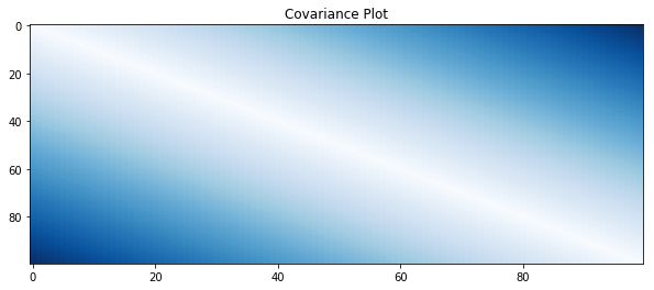
Finally, users may want to define their own kernels. This can be done with relative ease. It is left to the user to verify that the kernel they are using is in fact a valid kernel. This kernel can be anything from a simple numpy formula to a tensorflow neural network.
[25]:
# create new distance function
def new_distance_fucntion (alpha, beta):
    return np.abs(alpha - beta)

# define the kernel
kernel = kernel_base.Kernel(distance_function=new_distance_fucntion, method="k1")
[26]:
# create a vector
alpha = np.linspace(-2.0, 2.0, 100)
# get covariance
covariance = kernel(alpha, alpha)
[27]:
# plot covariance
plt.figure(figsize=(10, 4))
plt.title("Covariance Plot")
plt.imshow(covariance, cmap='Blues', interpolation='nearest', aspect='auto')
plt.show()
[ ]: